|
For this system, five local models were used, developed at input values
of 5, 10, 15, 20, and
![]() .
Linear state-space models were developed
at of these operating points using a Jacobian linearization of the process model.
Other types of models or methods for model development could be used. The
filter time constant for adjusting model weights was chosen as 4 minutes. This
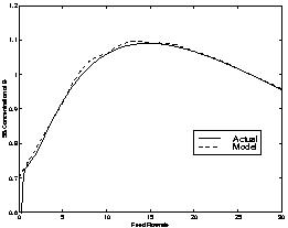
value is typical of the open-loop process system. A steady state comparison
of the actual model and the multiple model is given in Figure 5.
This shows that at steady-state there is very little modeling error. At the
linearization points, the modeling error is zero. The greatest amount of error
is found away from the linearization points, between the selected modeling points.
In Figures 6 and 7, the frequency dependent
amplitude ratios and phase angles of the linearized nonlinear system model are
shown for various operating points. The input levels displayed include the five
input values as well as operating points between the five operating points.
The amplitude ratio displays the expected gain approaching zero near the optimal
operating point. The phase angle plots show the inverse response models rolling
off to -270 and the non-inverse response models rolling off to -90 as expected.
.
Linear state-space models were developed
at of these operating points using a Jacobian linearization of the process model.
Other types of models or methods for model development could be used. The
filter time constant for adjusting model weights was chosen as 4 minutes. This
value is typical of the open-loop process system. A steady state comparison
of the actual model and the multiple model is given in Figure 5.
This shows that at steady-state there is very little modeling error. At the
linearization points, the modeling error is zero. The greatest amount of error
is found away from the linearization points, between the selected modeling points.
In Figures 6 and 7, the frequency dependent
amplitude ratios and phase angles of the linearized nonlinear system model are
shown for various operating points. The input levels displayed include the five
input values as well as operating points between the five operating points.
The amplitude ratio displays the expected gain approaching zero near the optimal
operating point. The phase angle plots show the inverse response models rolling
off to -270 and the non-inverse response models rolling off to -90 as expected.
From Figure 8, one can see that the multiple local
models overlay the actual models in most dynamic simulation cases. The nonlinear
model fits both the dynamics and steady-state values of the actual process.
A comparison with a single linear model (modeled close to the optima,
![]() )
shows that both the steady-state values as well as the dynamic response of the
linear model were inaccurate. The multiple linear model correctly predict inverse
and non-inverse response, depending upon the input levels and recent operating
conditions. The multiple model approach does exhibit a slightly under-damped
behavior in some cases where the actual model does not. This can be attributed
to the fact that the multiple model approach does not switch to new models quickly
enough in some situations.
)
shows that both the steady-state values as well as the dynamic response of the
linear model were inaccurate. The multiple linear model correctly predict inverse
and non-inverse response, depending upon the input levels and recent operating
conditions. The multiple model approach does exhibit a slightly under-damped
behavior in some cases where the actual model does not. This can be attributed
to the fact that the multiple model approach does not switch to new models quickly
enough in some situations.
Results from closed-loop simulations also appear promising (see Figure 9).
Here, various step changes in the process setpoint are given to the system.
The control system successfully tracks the setpoint at many different levels.
One of the linear controller responses (from model 5,
![]() )
demonstrating linear controller limitations is shown for comparison in Figure
9. The nonlinear system is more aggressive than a single
linear controller. When given an unobtainable setpoint, the nonlinear controller
finds a steady-state near the optimal value. The linear controller destabilizes
when faced with an unreachable reference. The nonlinear controller is winding
up error and will take some time to track a new feasible reference value. The
manipulated input does not constantly remain on one side of the process optima
in this example, managing to cross the optima and make use of all the system
models. In all simulation cases, input level constraints of 0 and 60 were enforced.
)
demonstrating linear controller limitations is shown for comparison in Figure
9. The nonlinear system is more aggressive than a single
linear controller. When given an unobtainable setpoint, the nonlinear controller
finds a steady-state near the optimal value. The linear controller destabilizes
when faced with an unreachable reference. The nonlinear controller is winding
up error and will take some time to track a new feasible reference value. The
manipulated input does not constantly remain on one side of the process optima
in this example, managing to cross the optima and make use of all the system
models. In all simulation cases, input level constraints of 0 and 60 were enforced.
Disturbance rejection was also tested. In this example, the cooling water flowrate
dropped from 10.5 to 5.0 at time=100. As one can see in Figure 10,
the nonlinear control system moves to reject this disturbance. This disturbance
results in a new system with an optimal value for the concentration of B below
the system setpoint. The multiple model control system moves to correct as much
as possible. If the disturbance is persistant, the integral action for the controller
eventually causes problems in the system since the reference is now unreachable.