Methodology

In process systems where a linear model or controller proves insufficient, it is desirable to have a simple representation that can model or control the nonlinear system. This leads one to consider a multiple model approach. There are many possible routes to take depending upon how much is known about the system.

• For this work, it is assumed that a first-principles model of the system under consideration is not known, although a first-principles model is used for simulation purposes.
• It is also assumed that the system does not exhibit output multiplicity. This implies that there could be input multiplicities in the process, resulting in a process optima with zero-gain.
• One final assumption is that local models may already be available for some operating conditions, while new models can be developed at other operating points.

To best piece together multiple local models, one must devise a method for partitioning the operating space for the system. For input multiplicity systems, it makes sense to partition the space using the system's input values. Operating points for the local models are chosen with regard to what existing models may be available, the known process characteristics (such as process optima), and the desired system operating range. In the next step for developing a multiple model system, one must assume a method for weighting the independent local models. In order to adequately capture steady-state values, a linear interpolation scheme is used in this work. This means that the model weights are based on the nearest two local models in the SISO case. When operating exactly at the point where the model i was devised, the weight for model i should be equal to 1. When operating halfway between two models each model should be weighed equally, resulting in weights of 0.50. This model weighting scheme removes the problems often associated with the normalization of overlapping basis functions as presented in [Murray-Smith and Johansen(1997)]. 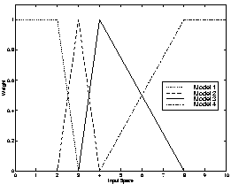The tail of a Gaussian model weight can extend well into another model regime, causing a model to become active in the wrong region. Typical model weights for the presented work are shown in Figure 1. In this figure, the models would be established at the operating points 2, 3, 4 and 8 in the input space of the system. This type of weighting has also been extended to a 2x2 MIMO case.

  

Figure 1: Model Weighting Function

Using the process inputs to select the correct operating point works well for steady-state analysis. When using this method of model switching, changes in the process inputs will cause the process to jump from one model directly to another. In order to allow for mixing of heterogeneous models, all local models are given absolute process inputs and produce absolute process outputs. As the process input changes from one value to another, the actual system does not respond immediately. This means that the actual state of the process is not moving instantaneously. 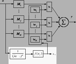To cope with this reality, the operating point for model switching is based on a filtered value of the system inputs. The filter is chosen with a time constant typical of the system. A second order filter with unity gain is used in this work. This creates a realistically smooth response that is continuously differentiable. 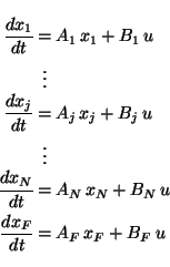See Figure 2 for a schematic. If one considers a linear state-space realization for each model M_j([A_j,B_j,C_j]), then the corresponding state-space composite model is given by:

$$\begin{eqnarray*}\frac{dx_{1}}{dt} & = & A_{1}\, x_{1}+B_{1}\, u\\ & \vdots & ... ...{N}+B_{N}\, u\\ \frac{dx_{F}}{dt} & = & A_{F}\, x_{F}+B_{F}\, u \end{eqnarray*}$$

$$\begin{eqnarray*}y & = & w_{1}(x_{F})\, C_{1}\, x_{1}+...+w_{j}(x_{F})\, C_{j}\, x_{j}+...\\ & & \, \, \, \, +w_{N}(x_{F})\, C_{N}\, x_{N} \end{eqnarray*}$$

where x_F corresponds to the states of the filter realization. Note that this model is a Wiener structure, and it is piecewise bilinear. Consequently, the rich literature on Wiener and bilinear systems is relevant to this approach.

  

Figure 2: Model Weighting Schematic

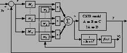
For control purposes, some work has to be done to make use of the model switching techniques. First, a controller must be devised for each local model. For this study, PI controllers were used for all local model controllers. These were tuned using IMC tuning rules and typical process reaction curve parameters. Use of IMC-PI form allows for a single tuning parameter for all controllers. The total system error is given to each controller. The output of each controller is multiplied by the current weights for each model. The total of all the weighted controller outputs is taken as the actual process input. See Figure 3.

  

Figure 3: Closed-loop Schematic